Next: O vetor de Poynting
Up: RADIAÇÃO
Previous: Os potenciais de Liénard-Wiechert
A personalidade dominante neste tópico é o grande Heinrich Hertz. As ondas de radio
eram conhecidas, pelos que falam difícil (como os locutores esportivos...) como
ondas hertzianas. Segue-se uma pequena biografia que copiei do livro de Sommerfeld,
Electrodynamics. É parte de uma coleção de física teórica, de 6 volumes, todos
esplêndidos, e de leitura deliciosa, pela riqueza de comentários humanos e
práticos que o orientador de Heisenberg, Pauli, Bethe, etc, gostava de incluir no texto.
Heinrich Hertz (1857-1894): he was born in Hamburg the son of a respected merchant
family; his father was in later years Senator of the Free City. Initially his great modesty
prevented Heinrich Hertz from entering the career of a scholar; instead, he turned to
engineering at the Technische Hochschule in Munich. Soon, however, he begged his
father to permit him to transfer to pure physics. He studied first in Munich, then in Berlin,
and became the favorite student and assistant of Helmholtz. A prize problem set up by
Helmholtz directed him to the testing of Maxwell's theory. After a short term as a
Privatdozent in Kiel he was called to the Technische Hochschule in Karlsruhe.
Even the earliest papers of Hertz show his mastery in relating theory and experiment.
Several of them received the warm recognition of his colleagues, as his quantitative
determination of hardness among engineers, and his description of the condensation
processes in rising air currents among meteorologists. His years in Karlsruhe, from
1885 to 1889, represent the high point in his creative activity. We mention in
particular his paper of 1888, Forces of electrical oscillations treated by Maxwell's theory. It
is amazing how much of the later development of radio telegraphy has been anticipated
in this paper. He is also the discoverer of the photoelectric effect, explained later by
Einstein in terms of photons, conceived then for the first time.
Trata-se de estudar a radiação eletromagnética produzida por uma fonte oscilante
localizada: um dipolo oscilante. Uma carga  está localizada na origem; uma carga
 oscila, em torno da origem, sendo
  seu vetor de posição. Então,
no momento
seu vetor de posição. Então,
no momento  , o momento elétrico de dipolo é
 |
(15) |
Em termos da notação usada na seção anterior,
 . Além disso,
 |
(16) |
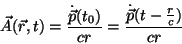
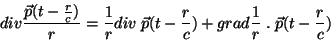
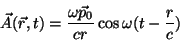
Podemos, portanto, construir imediatamente os potenciais. Usando a Eq.(14)
obtemos
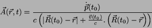 |
(17) |
com uma expressão análoga para  .
Vamos considerar o caso em que
.
Vamos considerar o caso em que
 |
(18) |
ou seja,
que dá
 |
(19) |
No movimento da carga positiva, a velocidade máxima alcançada é
 , onde
  é a sua distância máxima à origem. Então,
 |
(20) |
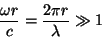
Supondo
 devemos então ter
 Vamos adotar esta aproximação, chamada aproximação de ondas longas.
Suporemos, além disso, que
Vamos adotar esta aproximação, chamada aproximação de ondas longas.
Suporemos, além disso, que
 , ou seja, que
estamos observando o potencial em pontos distantes da região ocupada
pelo dipolo. Nestas condições,
, ou seja, que
estamos observando o potencial em pontos distantes da região ocupada
pelo dipolo. Nestas condições,
 |
(21) |
e
 |
(22) |
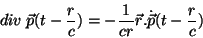
Logo,
 |
(23) |
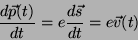
O cálculo de
 é delicado, pois temos de manter
a mesma ordem de aproximação. A maneira mais simples de fazer isso
é usar a condição de Lorentz,
é delicado, pois temos de manter
a mesma ordem de aproximação. A maneira mais simples de fazer isso
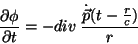
é usar a condição de Lorentz,
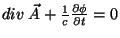 . Temos, então,
 |
(24) |
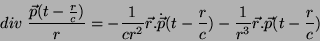
Logo,
 |
(25) |
Ora1,
 |
(26) |
Mas,
 |
(27) |
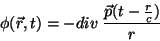
logo,
 |
(28) |
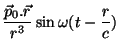
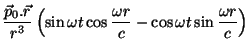
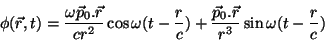
Concluíndo,
Pondo, em particular,
 |
(31) |
tem-se
 |
(32) |
e
 |
(33) |
e
 |
(34) |
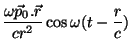
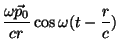
Suponhamos que  (zona de radiação). Então,
 |
(35) |
Na expressão para , a relação do primeiro termo para o segundo é da
ordem de
 , logo, para , o primeiro termo
é dominante. Então,
, logo, para , o primeiro termo
é dominante. Então,
No problema há três escalas de distância:  ,
,
 e
e  . Estamos sempre supondo que
 . Restam
então duas possibilidades a analisar: a primeira, já vista, é
quando , que é a chamada zona de onda, ou zona de radiação.
A segunda corresponde a
. Restam
então duas possibilidades a analisar: a primeira, já vista, é
quando , que é a chamada zona de onda, ou zona de radiação.
A segunda corresponde a  (mas ainda com
 ).
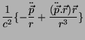
Neste caso, temos que
).
Neste caso, temos que
que é o potencial estático de um dipolo com momento variável. Os campos
obtidos são os campos estáticos
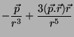
Na zona de radiação tudo é bem diferente:
Subsections
Next: O vetor de Poynting
Up: RADIAÇÃO
Previous: Os potenciais de Liénard-Wiechert
Henrique Fleming
2002-04-20